Read noise, Shot noise: The total noise in the raw data is a combination of all the above noise sources. Independent noise sources combine in quadrature -- that is, the square of the total noise is the sum of the squares of the individual contributions. The most important noise sources for typical exposures are read noise and photon shot noise. Together, they determine the signal-to-noise ratio available for given exposure parameters, and thus the image quality. Combined in quadrature, the read noise R and the photon shot noise P determine the total noise N as

      N² = R² + P²

ignoring the effects of thermal noise, PRNU, etc.

Poisson statistics dictate that the magnitude of photon shot noise is the square root of the number of photons; if S' is the number of photons in the signal, the typical number P' of photon counts attributable to shot noise is

      (P')² = S'

However, the pixel raw data is given by the raw value in ADU, rather than directly in terms of photons. The constant of proportionality between captured photons (or equivalently, photon-electrons in the sensel) and raw levels is the gain g. With g photons/raw level, one has signal S=S'/g and shot noise P=P'/g, where S is the signal in ADU and P is the shot noise in ADU. The gain is inversely proportional to the ISO setting; if one doubles the ISO and halves the exposure, half as many photons are captured but the raw value remains the same. Thus one has

      g = U/G

where G is the ISO setting, and U is a constant (which differs for different camera models) known as the unity gain.

The upshot is that the signal and shot noise measured in ADU are related by

      P² = S/g

Thus, read and photon shot noise contribute as

      N² = R² + S/g

where N, R and S are measured in raw levels (ADU).

Bottom line: One can measure both the read noise R and the gain g by measuring the noise in raw levels at a variety of exposure levels, plotting the square of the noise vs. the exposure, and fitting the result to a straight line; R is the square root of the intercept of this line, and g is the inverse of its slope.

Systematic effects such as PRNU, as well as subtle gradients across the image, can contaminate the measurement of read and shot noise. In order to eliminate these effects, the combined photon and read noise is best measured by taking the difference of two successive images having the same exposure level. The fixed systematic effects cancel between the two images when they are subtracted, leaving only fluctuations whose standard deviation is sqrt[2]~1.414 times the combined read and photon noise of a single image (because noise adds in quadrature, the noise of two images added together is N_sum=sqrt[N²+N²]=sqrt[2]*N ).

A uniformly illuminated, slightly out-of-focus GM colorchecker chart provides a suitable target image, with each square providing a uniform patch in which to measure the noise and signal levels, and thus several data points from a single image. Taking the images slightly out-of-focus helps ensure that any surface imperfections of the target do not give a false contribution to the noise measurements. Alternatively, one can take successive pairs of (completely out-of-focus) images of a blank, uniformly lit wall, or cloudless blue sky, incrementing the shutter speed from saturation to near black.

To summarize, the procedure is

1. Take a pair of images of a uniformly lit, slightly out of focus colorchecker chart.
2. Take the sum of the two images, and separate the result into its individual color channels. Measure the average raw value of each patch in one of the two green channel subarrays of the Bayer color filter array (or if desired, for each color channel). Divide by two (and, for Canon cameras, subtract the bias offset) to get the average signal.
3. Take the difference of the two images, split into color channels, and measure the standard deviation in each color patch. Divide by sqrt[2] to get the combined shot+read noise for that patch.
4. Plot the noise^2 vs. the signal, fit to a straight line. The intercept is the square of the read noise, the slope is the inverse of the gain.

The results for a Canon 20D are shown in Figure 9.

Fig. 9 - A plot of read+shot noise squared vs. exposure, from a Canon 20D at ISO 100, using pairs of shots of clear blue sky at varying shutter speed.
The intercept of the best fit straight line is the square of the read noise, while the slope is the inverse of the gain.   In this case, one finds the read noise R=2.5, and the gain g=11.6

On Canon DSLR's, there is an alternative method of measuring the read noise. Canon applies an offset or bias to the signal from the sensor; a constant voltage is added to the signal from the sensor before the signal is quantized in the ADC. Although voltage fluctuations can be either positive or negative, a fluctuation of negative amount will get clipped to zero upon quantization, since the output of the ADC is a non-negative integer raw value. By adding a bias or offset voltage, the full histogram of noise is preserved, since a small negative fluctuation from the offset value is still a positive number:

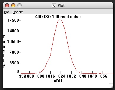
Fig. 10 - Histogram of a 40D blackframe. Canon applies an offset before quantizing the signal, amounting to 1024 raw levels for the 40D (and 1D3/1Ds3).
Without this offset, "black" values below the mean of the distribution would have been clipped.

When a bias is not applied (as for instance with Nikon cameras), negative voltage fluctuations are clipped to zero, making efforts to analyze and remove various forms of read noise more difficult. An example of this clipping is shown in figure 11.

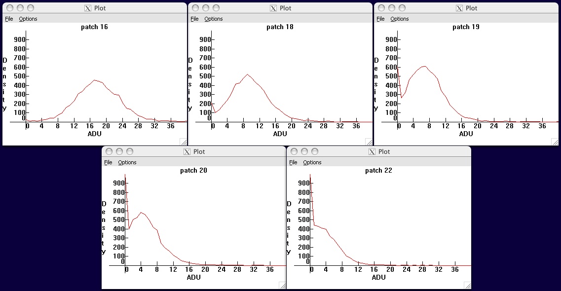
Fig. 11 - Noise histograms of a D300 as the exposure is lowered toward zero.   Voltage values below zero are clipped to the quantized raw value zero by the ADC,
leading to a spike in the histogram as all negative voltage values are digitized to the raw value zero. As a result, the standard deviations of blackframes underestimate the read noise.

PRNU: Pixel response non-uniformity (PRNU) is an additional effect which can be measured via the same technique just outlined. The non-uniformity turns out to be only a fraction of a percent, and consequently it is justifiable to treat this random variation in pixel response as another noise source to be added in quadrature to read and shot noise:

      N² = R² + P² + W²

where W is the contribution of PRNU, and as before N, R, and P are the total noise, read noise, and shot noise respectively. Now, PRNU is due to fluctuations in responsiveness of the pixels to light, and so the fluctuations it produces will increase in direct proportion to the illumination level S; in other words

      W = k S

where k characterizes the amount of variation in pixel responsiveness.

Read and shot noise were measured above using the difference of two identical exposures, in part to eliminate the effects of PRNU. A single test image will include the effects of PRNU as well as read+shot noise, the difference of two such images will have read+shot noise but not PRNU. Therefore, to measure pixel response non-uniformity, one simply measures the standard deviation of either of the two files used to determine read+shot noise, and subtracts out (in quadrature) the read+shot contribution previously determined:

      N² - (R² + P²) = W²

Bottom line: PRNU is expected to be linear as a function of the exposure, so plotting the values of W determined by this procedure vs. the corresponding raw values S should yield a straight line whose slope k is the fractional variation in gain from pixel to pixel.

It is important to choose a patch of the sensor relatively free of dust spots in order to get a good measurement -- dust spots will dim the response of the pixels underneath them and thus contribute a non-uniformity of response that looks just like PRNU. Similarly, the test image should be as uniformly illuminated as possible (and the measurements made on fairly small area patches) in order to eliminate as much as possible the effects of tonal gradients across the image, which will contribute to the width of the histogram but are not noise. For convenience, here again is Figure 7, plotting PRNU as a function of exposure for a 20D:

Fig.7 - Noise (denoted W in the text) due to pixel response non-uniformity of a Canon 20D at ISO 100, as a function of raw value
(denoted S in the text).   Mouse over to compare to the magnitude of combined read noise and photon shot noise.

Fluctuations in the response from pixel to pixel are given by the slope n=.006 of this curve; in other words, PRNU is about 0.6% for the camera tested.

S/N ratio vs. exposure, and Dynamic Range: Having measured the read noise and the gain, one can plot the signal-to-noise ratio versus signal at various ISO to get an idea of image quality in various exposure zones and ISO gains. At signal S, the combined read and shot noise are

      N = sqrt[R² + S/g]

At low signal, the read noise is more important; the noise is approximately constant and so S/N rises linearly with signal. At high signal, the photon noise is more important, and so S/N rises as the square root of signal. A plot of this behavior is shown in figure 12 for the Canon 1D3. When plotted on a log-log scale (i.e. in units of stops for both exposure and S/N), the linear rise at low exposure produces a slope approximately equal to one; then there is a "knee" in the curve, above which the square root relation between signal and photon noise takes over and the slope drops to one half.

Fig. 12 - Signal-to-noise ratio vs. exposure of the 1D3, for various ISO.   The horizontal axis is the raw value (signal) in EV
horizontal coordinate x corresponds to raw value S=2^x-1); (that is, the vertical axis is S/N ratio in stops (for S/N in dB, multiply by six).
Only read and photon noise have been taken into account in generating the above plot; PRNU and other noise sources are not incorporated.

Similar plots have been generated for the Nikon D3, Canon 1Ds3, Canon 5D, and Canon 40D. It should be emphasized that these plots take into account only read noise and shot noise, ignoring pattern noise and pixel non-uniformity, thermal noise, etc; these are safely ignored for exposure times of less than a second and ISO's of 400 and higher (and all but the highest exposure zones at ISO 200 or less). Note also that the visual effect of pattern noise outweighs its contribution to the noise statistics and may lead to a lower image quality than the S/N ratio might suggest.

We have so far not included PRNU in the considerations of S/N. In part this is because, as opposed to read and shot noise which are random, PRNU is fixed and can be known for a given camera sensor; thus it can be compensated for if desired (see page 4 of this article for a discussion) by multiplying each pixel value by a compensating factor according to its measured response variation. However, if one doesn't take such countermeasures, PRNU places an upper limit on the S/N ratio. Since the PRNU noise W is proportional to the signal S

      W = k S

and since the total noise N is larger than the PRNU noise W, the S/N ratio is bounded above by (cannot exceed) k. For instance, on my 20D, k=.006, and its S/N ratio saturates at log₂[1/.006]=7.4 stops; a 1D3 tested has a PRNU coefficient k=.0047 and so its S/N ratio saturates at log₂[1/.0047]=7.7 stops. The result of including the effect of PRNU on the S/N ratio plot of the 1D3 may be found here.

Bottom line: The inverse of the slope of the PRNU graph (see Figure 7 for an example) is an upper limit for the S/N ratio, unless PRNU is compensated for in post-processing.

The S/N ratio is closely tied to the dynamic range (DR) of the camera. The engineering definition of dynamic range is the maximum recordable signal (the raw value at which the sensor saturates) divided by the read noise, which is the lowest recordable signal. The raw value for sensor saturation cannot be assumed to be the maximum possible raw level, and must be measured (for instance by overexposing a scene by, say, five or six stops). For instance, on a Canon 40D tested at ISO 100, the sensor saturates at raw level 13825 rather than the maximum 14-bit value of 16383; the max signal is thus 13825-1024=12801 after subtracting the bias offset written into the raw data. The read noise at this ISO is 5.5 ADU, and so the dynamic range is 12801/5.5=2327, or 11.2 stops.

However, not all the dynamic range so obtained is useful in practice; the engineering definition assumes that any signal above zero is detectable and of sufficient quality to work with. A notion of practical or useful dynamic range may have more value than an engineering definition of dynamic range. However, what is useable to one viewer may be useless to another, allowing subjective judgment to enter into the DR standard. So, we leave it up to the viewer to decide for themselves and make their own standard for useful DR, with the aid of the following little tool. Figure 13 shows an image composed of the following ingredients:

• A tonal gradient spanning 32 levels on the 0-255 scale of 8-bit tonal depth.
• Text with tonal value equal to the minimum of the gradient.
• Read noise from a 1D3 blackframe, normalized to have standard deviation equal to four levels.

Fig. 13 - Text superposed on a tonal gradient, with superposed read noise. The contrast difference between text and background rises linearly across the image,
while the noise stays constant; thus the S/N ratio rises linearly from zero to eight going from left to right.

Having decided the minimum acceptable S/N ratio (if it's higher than 8, the reader is invited to generate their own S/N tool), return to figure 12 to determine the "useful" dynamic range. Locate the raw value where the S/N ratio meets your threshold for acceptability, then count the number of stops to the saturation raw level; this then is the useful dynamic range. For instance, suppose the minimum acceptable S/N ratio is 4=2²; on the 1D3, this S/N ratio is achieved for ISO 200 at roughly S=2^4.4, 9.5 stops below the saturation value of 13.9 (the max raw value is a bit less than 2¹⁴-1=16383 due to the bias offset of 1024). For ISO 3200, the same exercise gives a useful DR of about 7.1 stops (from 6.8 to 13.9).

Read noise vs. ISO: Read noise increases with ISO, because any noise added from the sensor readout before ISO amplification is then amplified by the ISO gain amplifier. A crude model of the variation of read noise with ISO is thus to assume independent pre- and post-amplification noise sources, that are combined as usual in quadrature:

      R² = (G R₀)² + R₁²

Here R is the total read noise; R₀ is the noise coming from circuit components upstream of the ISO amplifier, whose ISO gain is set to G; and R₁ is the noise arising from circuit components downstream of the ISO amplifier.

For example, the fit of this simple model to the read noise vs. ISO of the Nikon D3 is shown in figure 14 (data courtesy of Bill Claff). The parameters resulting from the fit are R₀=1.22 x 10 ^-2 ADU and R₁=4.2 ADU.

Fig. 14 - Read noise vs. ISO for the Nikon D3.   Points are data, courtesy of Bill Claff;
the curve is a fit to the read noise model presented in the text.

A similar plot for the Nikon D300 may be found here.

Nikon appears to use a single variable gain amplifier to implement all ISO settings, as is indicated by the D300 data (I don't yet have data on all intermediate ISO's for the Nikon D3). Higher end Canon models implement ISO gain via a two-stage amplification system; one amplifier for the "main" ISO's 100-200-400-800-1600 etc, and a second-stage amplification to implement the "intermediate" ISO's 125-250-500-1000 etc. and 160-320-640-1250 etc. The first amplifier amplifies the input noise, and adds some more noise of its own; the second amplifier amplifies the combined noises, and then adds some more noise. Combining all the noises in quadrature, the natural extension of the read noise model for two stages of amplification is thus

      R² = G₂² ((G₁ R₀)² + R₁²) + R₂²

where G₂=1, 1.25, 1.60 is the gain that generates the intermediate ISO's from the main ISO's, and G₁=100, 200, 400, 800, 1600, ... are the main ISO gains (the order of the amplifications could be reversed, but that arrangement turns out not to fit the data). The fit of the model to read noise data for the 1D3 is shown in figure 15 (data courtesy of Peter Ruevski)

Fig. 15 - Read noise vs. ISO for the Canon 1D3.   Points are data, courtesy of Peter Ruevski; the curves are a fit to the read noise model
presented in the text -- one set of curves holds G₂ fixed and varies G₁, the other holds G₁ fixed and varies G₂.

The fit parameters for the two-stage amplification model used in the plots are

	R0	R1	R2	sqrt[R12+R22]
1D3	0.82 x 10 -2	3.9	2.7	4.7
1Ds3	1.25 x 10 -2	5.1	2.4	5.6
5D	0.21 x 10 -2	1.6	0.9	1.9

Note that 1D3/1Ds3 data are in 14-bit ADU, while the 5D data are in 12-bit ADU, so to compare, multiply the 5D values by a factor of 4. For the main ISO's, the last column in the table combines (in quadrature) the contributions to the model from noise downstream of the main ISO amplification. In all cases, the downstream noise sqrt[(G₂ R₁)² +(R₂)²] dominates the read noise at low ISO, and the upstream noise R₀ provides the main contribution to read noise at high ISO. One sees in particular that the 1D3 and 5D have comparable high ISO performance at the pixel level, with the 1Ds3 trailing by about half a stop; and at low ISO, the 1D3 leads, followed by the 1Ds3 and then the 5D.

The two-stage amplification employed by Canon gives a bit more information as to what portion of the read noise can be attributed to different circuit components in its high-end cameras. Because of the second stage of amplification, one has separate information on how much of the read noise is due to noise in the main ISO amplification and how much is downstream from it in the secondary amplification and ADC. One sees from the table that the dominant noise at low ISO arises from the main ISO amplifier noise R₁, with a smaller contribution R₂ from the components downstream from this amplifier and a negligible contribution from the sensor readout noise R₀. Lower noise amplifiers would improve low ISO read noise and result in higher dynamic range at low ISO.

The read noise vs. ISO graphs show that, at some point around ISO 1600 to 3200, it ceases to make much difference whether the ISO gain is implemented as a hardware amplification or as a software multiplication of the highest hardware ISO. For instance, on the 1D3 the read noise 26.2 ADU at ISO 3200 is just about double the value 13.4 ADU at ISO 1600. This is why the so-called extended high ISO settings on Canon and Nikon (ISO 6400 on the 1D3, ISO 3200 on the 1Ds3 and 5D; all ISO's above 6400 on the D3) are implemented in software after digitization rather than as hardware amplifications -- the read noise will be the same, and its magnitude is so much higher than the quantization step that the "missing" levels after multiplying the raw values by 2, 4, 8, etc to make the extended ISO's have no effect whatsoever (they are once again dithered away by the noise). Photon noise, being a property of the light itself, couldn't care less what ISO is set in the camera; only the read noise enters into the question of whether the data amplification is as well done in software post-capture as it is by hardware during image capture.

On the other hand, if shooting raw, it makes little sense to use the extended ISO's since they are simply mathematical manipulations of the raw data post-capture, and their main effect is to throw away one or more stops of highlight headroom as the doubling, quadrupling etc of the raw values pushes more and more of them beyond the maximum recordable value of 4095 for 12-bit, or 16383 for 14-bit data. Setting the highest analog ISO amplification keeps the headroom, and one can always do as much additional software amplification as is needed afterward during raw conversion.