![]() ----------- Your trusted
source for independent sensor data- Photons to Photos------------------------ Last revised:
2017-05-16
----------- Your trusted
source for independent sensor data- Photons to Photos------------------------ Last revised:
2017-05-16
Previous Article----------------------------------- Table of Contents------------------------------------ Next
Article
-- Sensor Analysis Primer - Engineering and Photographic Dynamic Range
--------------------------------------------------------- By Bill Claff
Introduction
Engineering and Photographic Dynamic Range (PDR) can be read directly from a close relative to the Photon Transfer Curve (PTC).
The Photon Transfer Curve with a Twist
Here is a chart of the Photon
Transfer Curve for the Nikon D300 in ADUs at all whole ISOs based on 14-bit
ADUs:
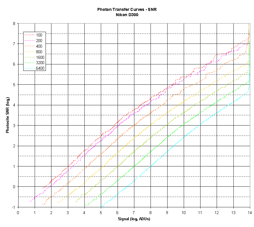
Note that for simplicity I am only showing the Gr channel from the Color Filter Array (CFA).
In this variation the y-axis is Signal to Noise Ratio (SNR) rather than the noise.
In my mind this is the single most important chart that characterized the performance of any sensor.
The data can be use to compute both Engineering and Photographic Dynamic Range.
Engineering Dynamic Range
The low endpoint for Engineering Dynamic Range is determined by where the SNR curve crosses the value of 1.
Here is an extreme close-up of that area of the Photon
Transfer Curve:
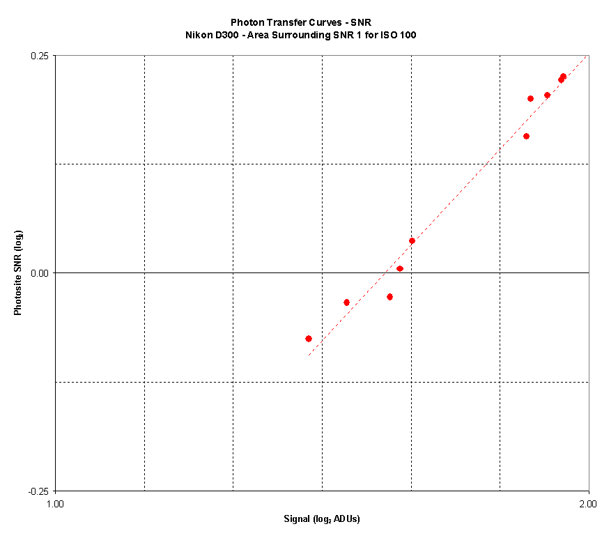
The ISO 100 line crosses 0 (the log2(1)) at 1.63 EV.
So Engineering Dynamic Range is 14.00 EV - 1.63 EV = 12.37 EV.
Or, if we use the White Level (from White Level), (14.00 EV - 0.11 EV) - 1.63 EV = 12.26 EV.
Photographic Dynamic Range
My definition of Photographic Dynamic Range is a low endpoint with an SNR of 20 when adjusted for the appropriate Circle Of Confusion (COC) for the sensor.
For the D300 the SNR values on this curve is for a 5.5 micron square photosite.
To correct for a COC of .022mm we are looking for a log2 SNR value of 2.49.
Here is an close-up of the area of the curve:
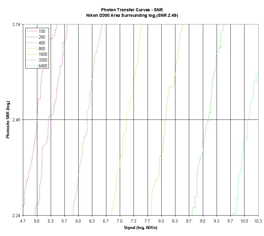
Note that the ISO 100 crosses 2.49 at 5.00 EV.
So Photographic Dynamic Range at ISO 100 is 14.00 EV - 5.00 EV = 9.00 EV.
Or, if we use the White Level (from White Level), (14.00 EV - 0.11 EV) - 5.00 EV = 8.89 EV.
Conclusions
Both Engineering and Photographic Dynamic Ranges computed in this article are slightly higher than those I report elsewhere.
The reason is that this analysis is because we only used the Gr channel from the Color Filter Array (CFA) and my reported values are across all channels.
Since the red and blue channels perform a little less well, the average across channels is lower.
Although the chart in terms of ADUs is of the most practical use it is important to remember the lessons learned in examining the electron-based Photon Transfer Curve.
As gain (ISO) is raised, fewer electrons are gathered; so in actuality it is the highlights that are lost.
When the data is shifted to recover the lost highlights then noise becomes apparent in the shadows.