
Noise, Dynamic Range and Bit Depth in Digital SLRs
by Emil Martinec ©2008
last update: January 11, 2010
restored and reposted with permission by Bill Claff: August 15, 2015
The Consequences of Noise
Noise, Dynamic Range, and Bit Depth:
Both Canon and Nikon have introduced a finer level quantization of the sensor signal in digitizing and recording the raw data, passing from 12-bit tonal gradation in older models to 14-bit tonal depth in newer models. A priori, one might expect this transition to bring an improvement in image quality -- after all, doesn't 14-bit data have over four times the levels (16384) compared to 12-bit data (4096)? It would seem obvious that 14-bit tonal depth would allow for smoother tonal transitions, and perhaps less possibility of posterization. Well, those expectations are unmet, and the culprit is noise.
In the absence of noise, the quantization of an analog signal introduces an error, as analog values are rounded off to a nearby digitized value in the ADC. In images, this quantization error can result in so-called posterization as nearby pixel values are all rounded to the same digitized value. An example is shown in Figure 16; here, an 8-bit grayscale image of a smooth tonal gradient was generated in Photoshop using the gradient tool. The bit depth was then truncated to five bits (32 tonal levels instead of 256) using two successive levels adjustment layers, the first one reducing the output range from 0-31 from an input range of 0-255, the one above it setting the input range to 0-31 and the output range from 0-255. Mouse over the gradient to see the posterization that results from bit depth truncation.
Fig. 16 - A gradient from 0-255 in 8-bit grayscale.
Mouseover to see the posterization that results from truncating the bit depth
to five bits.
In the absence of noise, having 8 times fewer available levels
is readily noticeable.
These two successive levels adjustments first compress the tonal range, truncating the lowest three bits; then the second levels adjustment layer restores the range of the gradient from black to white on your monitor. The histogram of the 8-bit and 5-bit gradients is shown as an inset in the figure. Clearly, in the absence of noise one wants the highest possible bit depth in order to have the smoothest possible tonal gradients.
Now consider the effect of noise on the tonal transitions. Noise amounts to random jumps of tonality between neighboring pixels; the bigger the noise, the larger the random jumps are. If the jumps are larger than the interval between successive quantized values of tonality, posterization effects will be rendered imperceptible by the noise -- the stepwise transitions of posterization (of magnitude 8 levels in this example) can't be discerned if the level is on average randomly hopping around between any pair of adjacent pixels by more than the spacing between levels (in our example, the random jumps are by 12 levels on average). The smoothing of transitions through the effect of noise, sacrificing spatial resolution for smooth but noisy transitions, is known as dithering. Figure 17 shows what happens when noise of standard deviation 12 levels is added to the smooth tonal gradient before the bit truncation to 5-bit tonal depth (where the smallest allowed jump in tonality is 8 levels on the 0-255 scale). The noise is more than sufficient to eliminate any trace of posterization.
Fig. 17 - A gradient from 0-255 in 8-bit grayscale,
with added noise of width 12 levels.
Mouseover to see whether posterization results
from truncating the bit depth
to five bits. Can you tell that one image has eight times fewer levels than the other?
Posterization can occur in the presence of noise, but only when the quantization step is substantially larger than the noise. Figure 18 shows the effect of decreasing bit depth on the noisy gradient, until eventually the noise is substantially smaller than the step size. Posterization becomes apparent when the quantization step sufficiently exceeds the width of the noise, the random jumps in tonality due to the noise are no longer able to dither the discrete jumps due to quantization.
Fig. 18 - When the quantization step sufficiently exceeds the noise, posterization re-emerges.
It is important that the noise is present before quantization of levels, as it is in the processing of the signal from the camera sensor, where the noise is contributed by the sensor electronics and by photon statistics, before the signal reaches the analog-to-digital converter. Attempting to dither tonal transitions through the addition of noise after quantization is much, much less effective, as one may readily verify by altering the order of bit truncation and noise addition in the above example. If the reader would like to tinker with the effects of noise and bit depth in creating smoother tonal transitions, the layered Photoshop .psd file used to generate the figures 16-18 may be found here.
Quantizing the signal from the sensor in steps much finer than the level of the noise is thus superfluous and wasteful; quantizing the noise in steps much coarser than the level of the noise risks posterization. As long as the noise exceeds the quantization step, the difference between the coarser and finer quantization is imperceptible. As long as noise continues to exceed the quantization step in post-processing, it doesn't matter how one edits the image after the fact, since any squeezing/stretching of the levels also does the same to the noise, which will always be larger than the level spacing no matter how it is squeezed or stretched. On the other hand, quantizing the signal in steps coarser than the noise can lead to posterization. Ideally, the noise should slightly exceed the quantization step, in order that roundoff errors introduced by quantization are negligible, and that no bits are wasted in digitizing the noise.
Raw data is never posterized. That does not mean, however, that posterization cannot arise through raw conversion and post-processing. The condition for the absence of posterization is that the noise exceed the quantization step; we have seen that compression of levels and bit truncation can reintroduce posterization (for instance, Figure 18 was generated by compressing levels more and more), and levels/curves adjustments as well as gamma correction involve compression of levels in some part of the histogram, effectively doing a levels truncation in some exposure zones. Resampling involves averaging over neighboring pixels, which can reduce the level of noise below the quantization step; noise reduction has a similar effect. Finally, 12- or 14-bit image data are displayed or output on 8-bit devices, implementing a substantial bit truncation. All these effects can introduce posterization where it didn't exist previously. When posterization does arise, one must reconsider the processing chain that led to it and try to find an alternative route that avoids it. The main point of emphasis here is that the bit depth of the raw data is never the culprit.
As an extreme example of how post-processing can undo the dithering effect of noise, consider applying a radius 5 median filter on the bit-truncated (5-bit) tonal ramp of Figure 16:

Fig. 17a - A median filter of radius 5 filters the noise and posterizes the tonal gradient of Figure 17.
One might be concerned that while smooth gradients do not suffer under bit truncation in the presence of noise, details do. Again this is not a problem. Figure 19 shows the text+gradient introduced in the discussion of dynamic range. Recall that the noise was four raw levels, so truncating the last two bits (down to 6-bit tonal depth) should have essentially no impact on the legibility of the text. To see whether it does, mouse over the image to reveal the original 8-bit image, mouse off to return to the 6-bit version. Throwing away the noisy bits has little or no effect on the ability to extract the detail in the image.
Fig. 19 - The gradient plus detail introduced above,
truncated to 6-bit tonal depth. Mouseover to compare to the 8-bit version.
The 6-bit image is very slightly darker in places, since the bit truncation can
result in slight shifts of the average tonality.
Can you tell that one image has four times fewer levels than the other?
The above example images were manufactured rather than photographed. This was done so that the effects being illustrated could be carefully controlled. For instance, one cannot have a tonal gradient smoother than a uniform, linear ramp of brightness, so this is the ideal testing ground. One of the major claimed improvements of 14-bit tonal depth was to allow smoother tonal transitions, but the increased bit depth does not help in the presence of noise. Nevertheless, the reader may have a nagging suspicion that somehow, real images might show improvement while these manufactured examples don't. To dispel that notion, consider Figure 20, a crop of a 1D3 image which was deliberately taken six stops underexposed. The purpose of the underexposure was to move the histogram down six stops, which means the highest six bits of the 14-bit raw data will be unused; the lowest eight bits are where all the image data reside, and that can be accurately displayed on our 8-bit computer monitors.
One of the two green channels of the raw data was extracted, and the tonal range 1020-1275 was mapped with a levels adjustment to 0-255 on the 8-bit scale (recall the bias offset of the 1D3 is 1024). The image looks a bit dark because no gamma correction has been done. The lowest two bits of the image data have been truncated -- effectively the 13th and 14th bits, the two least significant bits of the original 14-bit image data, have been removed. This bit-truncated image is what one would have obtained had the 1D3 been a 12-bit camera. Mouse over to compare this effectively 12-bit 1D3 image with the 14-bit original. Again it seems there is little to choose between the two. The reader is again invited to play with the full image and its bit truncation; feel free to download the 6-bit and 8-bit versions of the cityscape and play with them.
Fig. 20 - Green channel of a
6 stops underexposed 1D3 raw image, showing the lowest 8 bits = 256 levels
of the 14-bit data
after the last two bits have been truncated.
The 1D3's noise exceeds four levels, so this should cause no image
degradation;
mouse over to compare to the image made
from the lowest 8 bits without the truncation.
The histograms are inset at the lower right.
Curiously, most 14-bit cameras on the market (as of this writing) do not merit 14-bit recording. The noise is more than four levels in 14-bit units on the Nikon D3/D300, Canon 1D3/1Ds3 and 40D. The additional two bits are randomly fluctuating, since the levels are randomly fluctuating by +/- four levels or more. Twelve bits are perfectly adequate to record the image data without any loss of image quality, for any of these cameras (though the D3 comes quite close to warranting a 13th bit). A somewhat different technology is employed in Fuji cameras, whereby there are two sets of pixels of differing sensitivity. Each type of pixel has less than 12 bits of dynamic range, but the total range spanned from the top end of the less sensitive pixel to the bottom end of the more sensitive pixel is more than 13 stops, and so 14-bit recording is warranted.
A qualification is in order here -- the Nikon D3 and D300 are both capable of recording in both 12-bit and 14-bit modes. The method of recording 14-bit files on the D300 is substantively different from that for recording 12-bit files; in particular, the frame rate slows by a factor 3-4. Reading out the sensor more slowly allows it to be read more accurately, and so there may indeed by a perceptible improvement in D300 14-bit files over D300 12-bit files (specifically, less read noise, including pattern noise). That does not, however, mean that the data need be recorded at 14-bit tonal depth -- the improvement in image quality comes from the slower readout, and because the noise is still more than four 14-bit levels, the image could still be recorded in 12-bit tonal depth and be indistinguishable from the 14-bit data it was derived from.
Another point to keep in mind is that, while the raw data is not posterized, post-processing can make it so, as was seen in the noisy gradient example above. This is again true for the 1D3 cityscape image. Applying a radius 5 median filter brings out posterization in the 6-bit version, as one can see here; the 8-bit version is more robust against the median filter, as one can see here. However, something as simple as appending two bits with random values to the 6-bit version substantially eliminates the posterization, as one can see here.
S/N and Exposure Decisions:
A common maxim in digital photography is that image quality is maximized by "exposing to the right" (ETTR) -- that is, raising the exposure as much as possible without clipping highlights. It is often stated that in doing so, one makes the best use of the "number of available levels" in the raw data. This explication for instance can be found in a much-quoted tutorial on Luminous-Landscape.com. The thinking is that, because raw is a linear capture medium, each higher stop in exposure accesses the next higher bit in the digital data, and twice as many raw levels are used in encoding the raw capture. For instance, in a 12-bit file, the highest stop of exposure has 2048 levels, the next highest stop 1024 levels, the one below that 512 levels, and so on. Naively it would seem obvious that the highest quality image data would arise from concentrating the image histogram in the higher exposure zones, where the abundance of levels allows finer tonal transitions.
However, the issue is not the number of raw levels in any given segment of the raw data (as measured e.g. in stops down from raw saturation point). Rather, the point is that by exposing to the right, one achieves a higher signal to noise ratio in the raw data. The number of available raw levels has little to do with the proper reason to expose right, since as we have seen the noise rises with signal and in fact the many raw levels available in higher exposure zones are largely wasted in digitizing photon shot noise (there will be more to say about this in a moment, when we consider NEF compression).
Consider for instance the 1D3, exposed to the right at ISO 3200. Then consider taking the same image, with the same shutter speed and aperture, at ISO 1600. The latter image will be one stop underexposed according to the ETTR ideology. In particular, the idea that the benefit of ETTR comes from the "number of available levels" suggests that the image quality would be one stop worse for the ISO 1600 image than it is for the ISO 3200 image, since by being one stop down from the right edge of the histogram, fully half the available levels are not being used. However, as we have seen, noise is much more than two levels in all exposure zones at these ISO's, so the extra levels used in the ISO 3200 image simply go into digitizing the noise, and are thus of no benefit in improving image quality. In fact, the quality of the two images will be very nearly the same (rather than one stop different):
The proper reason to expose to the right comes from figure 12 on page 2, showing the rise in signal-to-noise ratio with increasing exposure. By increasing the number of photons captured, the S/N ratio improves, and the image quality improves directly in proportion to that improved S/N ratio. For instance, that ISO 1600 shot above, has one stop more highlight headroom than the corresponding ISO 3200 shot, and (assuming the shooting conditions allow) opening up the aperture by one stop or slowing the shutter speed by half will improve the S/N ratio while pushing the histogram one stop to the right. Shooting at lower and lower ISO continues to provide more highlight headroom, and thus higher and higher absolute exposure is possible, allowing higher and higher S/N ratio. The end result is that exposing to the right at the lowest possible ISO provides the highest image quality, but not for the reason usually given.
Now, the preceding discussion might leave the impression that, for a fixed choice of the shutter speed and aperture, it doesn't matter whether one has underexposed at lower ISO or exposed to the right at higher ISO. In fact it typically does matter, but the example above was specifically chosen such that the noise profiles of the 1D3 at ISO 1600 and ISO 3200 are very nearly the same when the difference in gain is accounted for, and so in that case it didn't matter which ISO was chosen as far as noise at fixed exposure was concerned. This is typically true at the highest ISO's; however, at lower ISO it does pay to choose the highest ISO for which clipping is avoided.
Somewhat counter-intuitively, for fixed aperture/shutter speed, it is best to use the highest possible ISO (without clipping highlights); this result is consistent with the ETTR philosophy, since using higher ISO pushes the histogram to the right if one thinks about things in terms of raw levels (ADU). However, the benefit from the use of higher ISO comes in the shadows, not in the highlights where "there are more levels"; to demonstrate that will require some more detailed analysis of the noise and S/N graphs on page 2.
The read noise vs. ISO graphs on
on page 2
exhibit noise (as measured in raw levels) increasing with ISO.
The observed values were accurately fit by the model presented
there; in its basic form, the model gives the read noise R as
R2 = (G R0)2 + (R1)2
in terms of the noise R0 coming
from circuit components upstream of the ISO amplifier, whose ISO gain
is set to G; and the noise R1 arising from circuit components
downstream of the ISO amplifier.
The effect of increasing the ISO gain G emphasizes the contribution
of the upstream noise component, because it gets multiplied by a bigger
and bigger number the higher the ISO gain, to the point that at high ISO
the read noise is almost entirely due to upstream noises, with a
negligible contribution from downstream noises.
The noise measured in ADU is so-called output referred noise, the noise
in the output raw data after all the amplification etc that goes on in
the signal processing chain. It is sometimes useful to refer the noise
back to its input equivalent, in photoelectrons at the photosite, in order
to compare it to the photon noise or the signal, both of which are measured
in photoelectrons. This is accomplished by multiplying
by the gain g=U/G , the conversion factor between electrons and ADU; here,
U is a constant (the so-called universal gain) and G is the ISO setting.
When this is done, the opposite trend is observed --
read noise goes down with ISO in electron equivalents:
(R in electrons)2 = [ g * (R in ADU) ]2 =
U2 (R02 + R12/ G2)
The reason for this decrease is the decreasing influence of
downstream noise R1 with amplification; in referring the noise back
to input equivalents, the downstream noise gets divided
by the ISO gain, and hence becomes smaller and smaller at high ISO,
while the upstream noise didn't know about any amplification
and remains constant in input-referred units.
Bottom line: Read noise at high ISO is much smaller than read noise at low ISO, in terms of the error in photon counting that it represents. Thus, better image quality is obtained for using the highest ISO for which the signal is not clipped.
One sees this trend clearly when plotting the photon equivalent of read noise as a function of ISO:
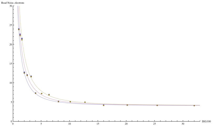
Fig. 15a - Read noise vs. ISO for the Canon 1D3 in photoelectron
equivalents.
Points are data,
courtesy of Peter Ruevski; the curves are a fit to the read noise model.
For the purpose of making exposure decisions, a variant of the S/N plots of Figure 12 is useful. In that set of graphs, the S/N ratio was plotted as a function of raw level. But raw levels mean different things for different ISO, so for the purpose of deciding which ISO to use it is more helpful to plot the S/N curves all normalized to the same exposure:
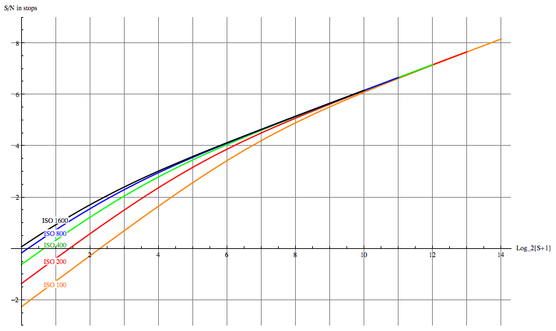
Fig. 12a - Signal-to-noise ratio of the Canon 1D3 for various ISO, as a function of normalized exposure value.
There are several ways to interpret this graph that are useful to keep in mind for making exposure choices. If one has the option to lower the ISO and the shutter speed (or widen the aperture), the highest S/N for the image is obtained by increasing the exposure, pushing the right end of the histogram right up to the upper edge of the range of exposure on the horizontal axis. This is the usual ETTR philosophy. Lowering the ISO one stop pushes the upper end of the dynamic range one stop to the right in absolute exposure, and pushing the histogram to the right climbs the rising S/N curve to better overall image quality.
If on the other hand, one is limited by the subject matter (freezing motion, depth of field requirements, etc) to a given maximum EV, then it makes sense to raise the ISO to pull the top end of the camera's dynamic range down to the top end of the histogram; this has little benefit at that upper end, since all the curves are on top of one another in that regime. Nevertheless it improves image quality by raising the S/N ratio on the shadow end of the curves.
Note that the expansion on the bottom end of the range yields less and less as ISO is increased more and more -- going from ISO 100 to ISO 200 yields a big improvement at the lower end of exposure (at the cost of some latitude at the upper end); on the other hand, going from ISO 800 to 1600 doesn't make much difference at all in shadow S/N, and in addition one loses an entire stop of raw headroom. Above ISO 1600 there is no expansion of the shadow range whatsoever, just more and more lost from the top end. The ISO 3200 curve of the 1D3 isn't even plotted above, because it lies almost exactly on top of the ISO 1600 curve, apart from ending one stop earlier ot the top end. This is why it makes no sense to use absurdly high ISO's like 6400 if one uses raw capture -- it just throws away highlight headroom without getting anything back at the shadow end; it's better to underexpose by a stop or two at ISO 1600 if the shutter speed is needed, than to use higher ISO.
It ceases to make sense to raise the ISO beyond 1600 on the 1D3 in raw capture, because there is no improvement in read noise measured in electrons; one loses highlight headroom with no compensating gain at the shadow end. (The bit depth is far more than is needed given the noise level in ADU.) It is better to underexpose at ISO 1600, since one obtains the same shadow detail with more highlight headroom, provided the raw converter can accurately apply the needed exposure compensation. For the same reason, there is little reason with Canon DSLR's to use the "intermediate" ISO's 500, 640, 1000, 1250 (and only minimal benefit to ISO 125, 160, 250, and 320), since their read noises are nearly the same as the next lowest "main" ISO of 100, 200, 400, or 800. Again, underexposure at that next lowest "main" ISO has almost identical shadow detail in the raw data, but delivers more highlight headroom. Nikon uses a different means of obtaining intermediate ISO's, such that the read noise drops more uniformly with increasing 1/3 stop ISO settings.
Bottom line: High exposure zones and/or high ISO, where photon noise and pre-amplification read noise dominate the noise, are rather insensitive to what ISO is chosen once a choice of exposure is selected and care is taken not to clip highlights. Underexposing by a stop, and doubling the raw values in post-processing (that is, applying exposure compensation), yields the same image quality as 'proper' exposure under these conditions. On the other hand, in lower exposure zones at low ISO, where post-amplification read noise becomes important, the read noise goes down by a bit less than a factor of two (in electrons) when the ISO doubles. In this situation, underexposing by a stop and doubling the raw values in post-processing, yields more noise than proper exposure, particularly in shadows.
By the way, underexposing at lower ISO is precisely what Canon cameras do in the raw data when Highlight Tone Priority (HTP) is enabled; and what Nikon cameras do when Active D-Lighting (ADL) is enabled. Instead of using the ISO gain set by the user, the camera uses a lower ISO (but exposes with the indicated aperture and shutter speed), effectively underexposing the image; this provides more highlight headroom. In post-processing, the image data can be brought back up while preserving the highlights with a modified tone curve in higher exposure zones. The place where image quality suffers is in shadows at lower ISO, precisely as the above quantitative model predicts.
An aside on "lossy" NEF compression:
The fact that level quantization much finer than the noise is superfluous, since noise erases the perceptual impact of abrupt tonal transitions, means that many of the levels used to record higher exposure zones are unneeded and indeed wasteful -- photon shot noise is much larger than the level spacing in midtones and highlights on a typical DSLR.
That is, if the average photon count is 10000, there will be fluctuations from pixel to pixel of as much as sqrt[10000]=100 photons in the sample. Suppose each increase by one in the raw level corresponds to counting ten more photons (i.e. the gain g=10 photons/ADU); then noise for this signal is 100/10=10 raw levels. The linear encoding of the raw signal wastes most of the raw levels, since the noise is much larger than the quantization step.
In shadows, it's a different story. Suppose our average signal is 100 photons; then the photon fluctuations are sqrt[100]=10 photons, which translates to +/- one raw level for the supposed gain g=10. At low signal level, none of the raw levels are "wasted" in digitizing the noise.
Ideally, what one would want is an algorithm for thinning the level spacing at high signal, while keeping it intact for low signal, all the while keeping the level spacing below the noise level for any given signal (to avoid posterization). Nikon's NEF "lossy" compression uses a lookup table to do just that, mapping raw levels 0-4095 (for 12-bit raw) into compressed values in such a way that there is no compression in shadows, but increasing thinning of levels for highlights, according to the square root relation between photon noise and signal. The uncompressed digitized raw value is rounded to the nearest value in the lookup table. The amount of compression increases as the uncompressed raw value increases above some threshold, in the same way that photon noise increases with illumination level.
Fig. 21 - Plot of a lookup table for NEF compression
(the particular lookup table is model-dependent, but all have
this basic structure).
The horizontal axis is the NEF compressed raw value; the vertical axis is the
uncompressed 12-bit raw value that it corresponds to.
Raw values that do not
correspond to a compressed value are rounded off to the nearest compressed value.
The blue curve is a plot
of the compression table, the red curve is the best fit
parabola to the nonlinear part of the compression table, as suggested by
the growth of photon noise masking level transitions.
The idea behind "lossy" NEF compression is thus to thin the levels in highlights where levels are too finely distributed relative to the inherent noisiness of light, but keep most or all of the levels in shadows where the magnitude of the noise fluctuations is smaller. This is why the NEF compression table is linear at the low end, and quadratic further up. The quadratic part is a reflection of the quadratic relationship between noise and signal of light (the noise squared is proportional to signal) -- the higher the signal the more levels can be thinned out. The linear part of the compression table kicks in when the signal is low enough that the noise fluctuations are less than or of order one raw level -- then no compression is possible and the output value must equal the input value.
Quantitatively, the appropriate criterion is that a jump in the compressed
value C by one should correspond to a span of raw values S
that is less than the noise (which is at least as big as the shot noise
sqrt[S/g]), so that the noise continues to dither the larger
jumps of the compressed image data where levels have been eliminated.
In other words,
dC > dS/sqrt[S/g]
A bit of calculus then leads to the relation between compressed values
and raw values
S < [(C-C0)2]/4g
where C0 is a constant offset equal to half the length of the linear
part of the table, where compression is not possible.
The best fit parabola to the nonlinear part of the lookup table,
which is the red curve in Figure 21,
has C0=134 and g=18. The criterion that the jumps
in compressed values not exceed the photon noise is that this value of
g should be more than the actual gain of the camera at its
base ISO. In fact, the typical base ISO gain for the Nikon models that use
this particular lookup table is about 6-8, so the
condition is met with a good margin of safety.
Bottom line: The "lossy" form of NEF compression is a clever use of information theory to save space by eliminating redundant raw levels. The noise which is unavoidably present in light effectively dithers tonal transitions so that the compression is lossless in that the image is still encoded without loss of visual information. In this sense, "lossy" compression is perhaps an inappropriate appelation.
Amusingly, Nikon engineers seem to have forgotten the logic behind the thinning of raw levels when upgrading to 14-bit tonal depth -- the NEF compression table has roughly four times as many entries (2753) for the 14-bit table as it does (689) for the 12-bit table in the D3 and D300, even though there is no purpose to the extra values given the relation between noise and quantization step in efficient data encoding.
-- How to compare noise and dynamic range --
The noise and dynamic range statistics
typically reported for cameras (and in particular those reported above)
are based on measurements for individual pixels.
The question then arises, how does one compare
noise statistics among cameras with different pixel sizes, different numbers
of pixels, and different formats (sensor sizes)?
The issue arises because, in general, smaller pixels are noisier.
Why is this so? Consider combining a 2x2 block
of pixels into a "superpixel" of twice the size. The raw value is proportional
to the number of photons collected; combining pixels, the photon counts add
and so the raw values should be added together:
S = S1 + S2 + S3 + S4
The noises combine in quadrature:
N = sqrt[ (N1)2+(N2)2
+(N3)2+(N4)2 ]
If the raw values are approximately equal, and the noise contributions are
approximately equal, the aggregate signal is four times that of the individual
pixel; on the other hand, the aggregate noise is about twice the noise of the individual
pixel. Thus the "superpixel" of four pixels binned together has twice
the S/N ratio of any of its component pixels. The effect
of combining pixels becomes somewhat more complicated in regions
where the image has texture or detail, since the noise fluctuations
Ni
in pixel values are being averaged together with tonal variations
in the signal values Si. The local variation of the measured
pixel values is some part noise, some part signal, and so the quantitative
reduction in the variation of pixel values will not give directly
the amount of noise eliminated, and the decrease in
the standard deviation of pixel values relative to average signal
will in general fall short of a factor of two.
Bottom line: At the cost of having half the linear resolution, the superpixel made by binning together a 2x2 block of pixels has up to twice the signal-to-noise ratio.
But wasn't this S/N ratio already there before we started binning pixels together? Of course it was. All we did by combining pixels was to throw away resolution. The point is that noise, and signal-to-noise ratio, are dependent on the spatial scale at which they are measured. Typically, S/N will be twice as large at twice the spatial scale, as the binning example demonstrates.
Another simple demonstration shows the scale dependence of noise:
There is little difference in this regard between shrinking the size of the image by downsampling -- which reduces the resolution by the percentage of shrinkage -- versus keeping the image size fixed and applying a blur, which again reduces the resolution by the ratio of the blur diameter to the pixel spacing. Either way one is averaging over pixels of the original image, and that reduces noise.
The conclusion is that noise is resolution dependent. If one compares two cameras having the same sensor size and technologies but different resolutions (pixel densities), the one with the lower resolution (lower pixel density) will have less noise at the pixel level, as the above exercise again demonstrates.
The same reasoning holds true when comparing two different camera models with different size pixels. All other things being equal -- the percentage of pixel area active in light collection, the efficiency of the pixels, etc -- the number of photons collected will be proportional to the pixel area (the square of the pixel spacing), while the photon shot noise will scale as the pixel spacing. So for example, the Canon 40D has 5.7 micron pixels, its gain (the number of photons collected per raw level) is 3.1 e-/14-bit ADU at ISO 400; the number of electrons collected per raw level per square micron is 3.1/5.7^2=.095. The Canon 1D3, on the other hand, has 7.2 micron pixels and a gain of 5.0 e-/14-bit ADU at that ISO; the light collecting efficiency per unit area is .097, essentially the same (the difference of the measured values is of order the variation from copy to copy of the same model). Using the same technology, Canon achieved the same light collection efficiency per unit sensor area for both cameras. As a consequence, the photon noise at fixed spatial scale is the same for both cameras.
Light collecting efficiency translates into photons, photon counts determine photon shot noise, and photon noise is the dominant noise source in highlights. The bigger pixels of the 1D3 collect more photons than the 40D, and this is reflected in the S/N ratio plots above (40D here, 1D3 here); at saturation signal of about 214, the S/N ratio of the 1D3 at ISO 200 is somewhat over 7.6 stops, the 40D about 7.3 stops. However, an ideal resampling of the image of one sensor to the pixel density of the other would yield the same photon noise, because the sensors capture the same light per unit area. Collection efficiencies of various sensors on a per area basis are tabulated in Table 1 (data from various sources -- Roger Clark, Bill Claff, Christian Buil, Bart van der Wolf, Peter Facey, and the author).
|
10D |
1D2 |
D200 |
5D |
350D |
1Ds2 |
20D |
400D |
D300 |
40D |
1D3 |
1Ds3 |
50D |
D3 |
|
.042 |
.049 |
.054 |
.061 |
.064 |
.064 |
.076 |
.083 |
.089 |
.095 |
.098 |
.098 |
.100 |
.113 |
Table 1: Light collecting ability per unit sensor area
of various camera models: 12-bit
gain at ISO 400 divided by pixel area in square microns.
(Note: Canon ISO calibration on earlier (12-bit) models such as the 1D2, 5D, 20D, 350D etc was understated by 1/3 stop; consequently, to fairly compare the above numbers, the efficiency per unit area should be multiplied by 1.25 for these cameras.)
The figures for light collection performance per unit area in the above table refer the sensor efficiency to a fixed spatial scale rather than considering it at the pixel level, and so accounts for varying pixel size among cameras. Fixed spatial scale is the appropriate metric for comparing different pixel densities if one takes the same image from two cameras with different pixel densities, at the same focal length. Taking equivalent crops from each camera, and resampling the image to the same print dimensions, the photon noise will be the same. A different metric will arise if one compares not to fixed absolute size on the sensor, but as a percentage of frame size; that will be considered below.
Thus photon noise at fixed spatial scale is independent of pixel size for a given per area collection efficiency. What about read noise? In order for read noise at fixed spatial scale to be independent of pixel size, read noise per pixel must decrease in proportion to pixel spacing -- if the pixel spacing is halved, there are four pixels in the area formerly occupied by one, with an aggregate read noise in that area twice that of the individual half-size pixels again, since noises combine in quadrature). Therefore, the half-size pixels must have half the read noise in order that the total read noise at the scale of the original pixels is the same.
The situation is somewhat subtle, however. The read noise varies with ISO, as the data and model presented on page 2 indicates. So at the very least one should examine the issue for each ISO, since the conclusions could be different for low ISO versus high ISO.
Consider the 40D and 1D3. At ISO 100, the 1D3 read noise is 4.8 ADU, while the 40D read noise is 5.5 ADU; at ISO 1600, the read noise is 13.4 ADU for the 1D3 and 22.6 ADU for the 40D. A similar disparity of read noises holds for the Nikon D3 and D300; both the larger pixel D3 and the D300 have about 5 14-bit ADU of read noise at lowest ISO, but the D3 has much lower read noise at high ISO.
However, noise figures in ADU mean different things for different cameras due to their differing efficiencies, and as discussed above different size pixels entail different levels of resolution which also affects the amount of noise observed in an individual pixel. So the question arises as to how these numbers should be compared. One way to normalize them is to compare relative to photon noises, and to the signal in photons, by converting the read noise values in ADU to their photoelectron equivalents. To convert read noise in ADU to photoelectron equivalents, one multiplies by the gain in electrons/ADU. For instance, the gain of the 40D is 3.1 electrons/14-bit ADU at ISO 100, while the 1D3 gain is 5.0 electrons/14-bit ADU at that ISO (for ISO 1600, divide these numbers by 16, since the gain value is inversely proportional to ISO). Then the ISO 100 read noises are 17 electrons for the 40D, and 24 electrons for the 1D3; the ISO 1600 read noises are 4.4 electrons for the 40D, and 4.2 electrons for the 1D3.
A second correction should be made for the differing pixel sizes. To normalize the noise of different size pixels one should rescale by the pixel spacing to refer them to the same spatial scale. When measuring noises in electrons, this normalization divides the read noise by the pixel spacing (bigger pixels means fewer per unit area, so fewer noises to combine). Thus at ISO 100, one compares 17/5.7=3.0 for the 40D, to 24/7.2=3.3 for the 1D3; at ISO 1600, one has 4.4/5.7=.77 for the 40D, and 4.2/7.2=.58 for the 1D3. On a per area basis, the smaller pixels do better than the larger ones at low ISO, while the larger pixels do better than the smaller ones at high ISO.
Naively, the above results would seem to suggest a slight dynamic range advantage for small pixels at low ISO, compared to a slight low light advantage to big pixels at high ISO. Further evidence for this trend will be found below when much smaller digicam pixels are compared to those of the 1D3. This reversal of fortune between low and high ISO is nicely explained by the read noise model developed on page 2. Read noise decreases between low and high ISO for DSLR's, as is seen in Figure 15a above. On the other hand, for the tiny pixels in digicams, the read noise in electrons is practically independent of ISO. Furthermore, light-collecting efficiency tuns out to be largely independent of pixel size over a very wide range of pixel sizes, from the biggest DSLR pixels down to the smallest digicam pixels. Thus the dynamic range per area, which is the maximum light collection ability per area divided by the read noise per area, is largely determined by the read noise per area for which the comparison will be worst for DSLR's at low ISO and best for DSLR's at high ISO.
The factor that limits the low ISO performance of DSLR's turns out to be the limited dynamic range of the ISO amplifier and ADC components downstream from the sensor, and not the sensor itself; the analysis leading to this conclusion also leads to a simple proposal for recovering an extra two stops of dynamic range from current DSLR's. However, rather than devote space to developing that explanation and proposal here, since it would take us somewhat off the main topic, that discussion is deferred to a supplemental page to this article.
For comparing pixels on a patch of sensor of a given area, the normalizations given above are the appropriate ones. However, one is often interested in comparing the overall noise of the image coming from different sizes of sensors, so noise per area is less relevant that noise normalized to the image frame. Thus another metric for comparison is to consider the entire frame, and if comparing two different sensor formats (such as the 1D3 and 40D considered above), shoot with different focal lengths (say 130mm on the 40D and 160mm on the 1D3) so that the field of view is kept fixed. In the case of fixed framing, we should refer the noise characteristics not to a fixed spatial scale in microns, but rather to a fixed percentage of the frame height. An appropriate figure of merit is to divide the per pixel noise values by the frame height in pixels, again because the noise combines linearly in the number of pixels combined. The clear rule of thumb that emerges from such an exercise (not surprisingly) is that larger size sensor formats are less noisy than smaller size sensor formats. A simple example is the 40D relative to the 1D3; both are 10MP cameras, with 2592 pixels in the frame height, and so in this particular example the frame-referred noise levels are the same as the pixel-level noises, and these are lower (as measured in ADU) at all exposure levels and ISO's for the 1D3. The read noises are similar in photo-electron units, but the 1D3's bigger photosites capture more photons, hence have higher S/N ratio. Bigger sensors have higher S/N ratios, because bigger sensors collect more photons.
-- Extrapolating to tiny pixel sizes --
An amusing extrapolation of the analysis of the effect of pixel size results from consideration of digicam raw data. The Panasonic FZ50 is a 10MP superzoom digicam with RAW capability. An analysis by John Sheehy, as well as the author's rough measurements on this FZ50 raw file using the noise vs. exposure graphical method outlined on page 2, yields a gain g of roughly .29 photons/12-bit ADU at ISO 400. Dividing by the square of the 2 micron pixel size yields .072 photons per ADU per square micron, comfortably in the middle of the efficiency table above. However, just as the Canon ISO calibration was off for its earlier models, digicam ISO calibrations differ from those of DSLR's. Typical DSLR's leave about 3.5 stops between metered middle grey and raw saturation; digicams put middle gray about 0.5-1.0 stop closer to raw saturation, due to their lower dynamic range. This means that their ISO calibration is about 0.5-1.0 stops understated in relation to DSLR ISO calibration, and so the FZ50 efficiency figure is actually higher than .072 by a factor 1.4-2.0, making the FZ50 sensor among the most efficient per unit area in capturing photons of any digital camera sensor currently available! Of course the sensor is only about 5.5mm x 7.3mm in size, so the photon noise referred to the frame size is rather poor, as it is for any digicam; but the photon noise at fixed spatial scale in microns or millimeters, rivals or betters the 1D3, 1Ds3 and D3. If the FZ50 sensor could be scaled up to the size of full frame, it would indeed rival these cameras for photon shot noise performance; and the resolution -- the 2 micron pixels translate into a 216MP (!) full frame camera (of course, for many applications the actual resolution will be limited by diffraction and lens aberrations). It is currently unclear whether this performance could be maintained as the sensor is scaled up by a factor of nearly five in linear dimension -- practicalities of supporting electronics for the pixels, speed in readout and processing, etc, may make it difficult to maintain the FZ50's performance in a scaled-up version. Nevertheless, what should be clear from the preceding analysis is that there is virtually no difference in photon collecting efficiency over a very wide range of pixel sizes, from 2 microns to over 8 microns.
So a digicam sensor can rival or even exceed the performance of the best current DSLR's in photon capture efficiency, and thus shot noise performance. What about read noise? Naively one might expect that the read noise is a fixed cost per pixel, so more pixels per area mean more read noise. John Sheehy reports a read noise for the FZ50 of 2.7 ADU ~ 3.3 electrons at ISO 100; my rough measurements on the raw file linked to above yielded 4.5 ADU ~ 5.4 electrons of read noise. Let's compare this to the Canon 1D3 by referring to fixed scale. This means dividing the read noise per pixl in electrons by the pixel spacing. The 1D3 read noise is 1.2 12-bit ADU = 24 electrons at ISO 100, and the pixel spacing is 7.2 microns, so its read noise figure of merit is 24/7.2 = 3.3; the FZ50 read noise figure of merit is somewhere between 3.3/2.0 = 1.7 (Sheehy's measurement) and 5.4/2.0 = 2.7 (my measurement). So again the FZ50 is as good or better than the best DSLR's in read noise (fairly compared by referring to fixed spatial scale), at the lowest ISO's. The comparison gets even better if we again factor in the relative calibration of ISO between the two cameras. At high ISO, things are again reversed -- the 1D3 read noise at ISO 1600 is 3.4 12-bit ADU = 4.2 electrons, while the FZ50's is still about the same in electrons according to Sheehy. Now when dividing by the pixel spacing to refer to fixed spatial scale, the comparison substantially favors the big-pixel DSLR, even when the relative ISO calibration is accounted for.
The above DSLR/digicam comparison outlines the extremes of what may be possible with current or near-term technology, if digicam pixel densities were used to populate full-frame sensors. The fact that a digicam's performance is in the same ballpark as the best DSLR's when referred to fixed spatial scale, suggests that the problems with noise in digicams is not due to their ever smaller pixels, but rather it is due to their continued use of small sensors.
Bottom line: Among the important measures of image quality are signal-to-noise ratio of the capture process, and resolution. It was shown that for fixed sensor format, the light collection efficiency per unit area is essentially independent of pixel size, over a huge range of pixel sizes from 2 microns to over 8 microns, and is therefore independent of the number of megapixels. Noise performance per unit area was seen to be only weakly dependent on pixel size. The S/N ratio per unit area is much the same over a wide range of pixel sizes. There is an advantage to big pixels in low light (high ISO) applications, where read noise is an important detractor from image quality, and big pixels currently have lower read noise than aggregations of small pixels of equal area. For low ISO applications, the situation is reversed in current implementations -- if anything, smaller pixels perform somewhat better in terms of S/N ratio (while offering more resolution). A further exploration of these issues can be found on the supplemental page. Rather than having strong dependence on the pixel size, the noise performance instead depends quite strongly on sensor size -- bigger sensors yield higher quality images, by capturing more signal (photons).
The other main measure of image quality is the resolution in line pairs/picture height; it is by definition independent of the sensor size, and depends only on the megapixel count. The more megapixels, the more resolution, up to the limits imposed by the system's optics.